Our new approach uses system states and interaction types to reveal causal links in observational data that traditional methods miss.

For centuries, the goal of science has been to answer "why." Why does the weather change? Why do neurons fire in a specific pattern? Traditionally, finding these answers required controlled experiments: changing one thing to see what happens to another.

But in many fields, like geophysics, climate science, or neuroscience, we can’t always run controlled experiments. We only have observational data: records of what happened. Trying to find causality just by watching these records is notoriously difficult. It’s easy to confuse correlation (two things happening together) with causation (one thing making the other happen). Furthermore, standard methods typically provide a single, global measure of causality. This approach fails to capture the nature of complex systems, where relationships are rarely static; instead, they are dynamic and fluctuate depending on the system's state.

In a new paper, we introduce a new method for quantifying observational causality by states and interaction type. This approach resolves how interactions evolve across different states, revealing dynamic structures that conventional tools ignore. The full code is available in our GitHub repository.

Why averages can hide the real story

Think about city traffic. If you mix together data from 3:00 AM and 8:00 AM, you might conclude that traffic lights barely matter because at 3:00 AM the roads are empty. But during the rush hour, traffic lights can determine whether the city flows or locks up.

That’s the core idea: the “rules” of a system can change across regimes. In our paper, we call these regimes states. A state might mean “cold temperature” versus “hot temperature,” “brain at rest” versus “brain under cognitive load,” or “market calm” versus “market stressed.” When you average across all states, you can miss the most important causal story: the causal influence may be concentrated in specific states, and nearly absent (or even reversed) in others.

Our framework is built to detect exactly these differences: when causality is active, not just whether it exists on average.

Our perspective: causality as information about the future

We quantify causality as a simple question: how much does knowing the past reduce uncertainty about the future? Using information theory, we measure “causal influence” as information gained about a future outcome from candidate past drivers.

The key difference in our method is that we don’t compute a single average score. Instead, we evaluate this influence state-by-state. That lets us identify when causality is actually active — for example, identifying the specific states of a source variable that most strongly reduce uncertainty about the future state of the target (causal states), and separating them from states where the source is misleading (non-causal states). The rest of causality that cannot be explained from the sources comes from unobserved variables.

Three ways variables can drive the target

Furthermore, in complex systems, causes don’t always act alone. Often, the mechanism is in the combination of these variables. Our method captures this possibility by decomposing causal influence into different types of interactions.

Picture this: you’re trying to predict whether it will rain tomorrow, and you have a couple of measurements — two pressure sensors and humidity. Depending on how the atmosphere works in that moment, those signals can contribute to the forecast in three distinct ways:

• Redundant: both sensors tell you essentially the same thing, so either one is just as useful as the other.

• Unique: a sensor in a better location (for example, closer to the coast) picks up an incoming front earlier and adds information the other can’t.

• Synergy: pressure alone might be ambiguous, but low pressure together with high humidity becomes a much stronger indicator of rain than either measurement on its own.

A real-world example: the Walker circulation

We applied the method to a classic climate system: the Walker circulation. This system consists of a large-scale cycle of air movement across the tropical Pacific that helps shape global weather.

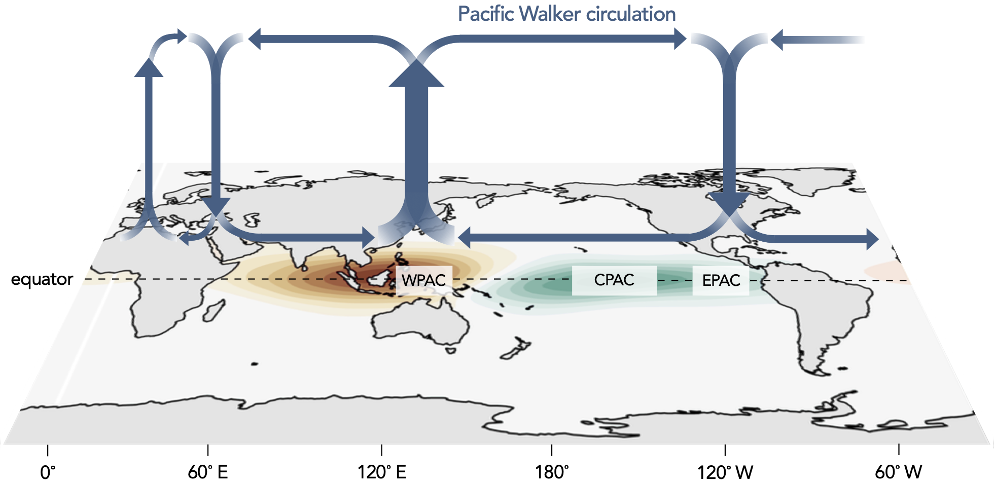
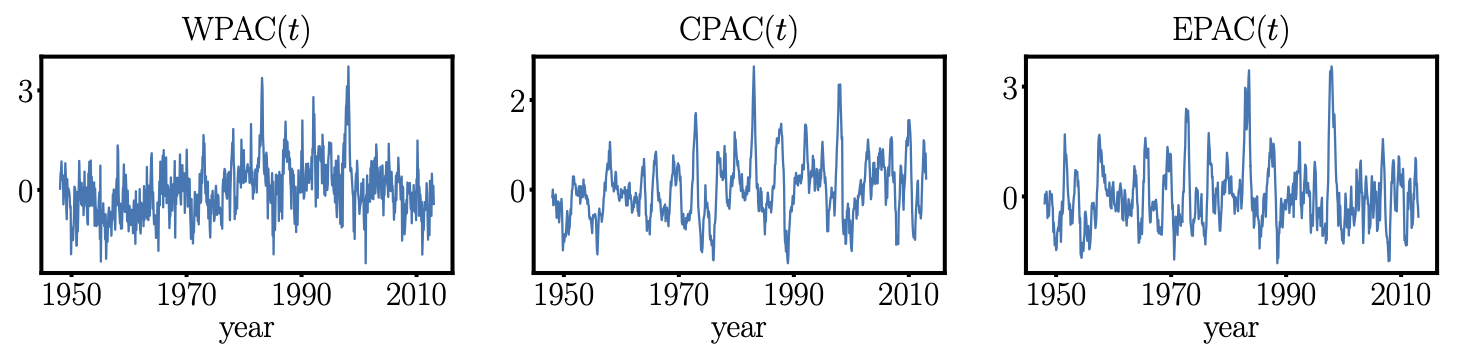
To analyze the interactions of variables within this system, we used monthly data from 1948–2012 (780 months), built from regional averages of:

WPAC: surface pressure anomalies in the West Pacific
CPAC: surface air temperature anomalies in the Central Pacific
EPAC: surface air temperature anomalies in the East Pacific

The key question to answer is: in which states do these variables drive one another? Below we show the causality maps produced by our method: instead of returning a single “causality strength,” the approach returns where in state-space the causal interactions concentrate.

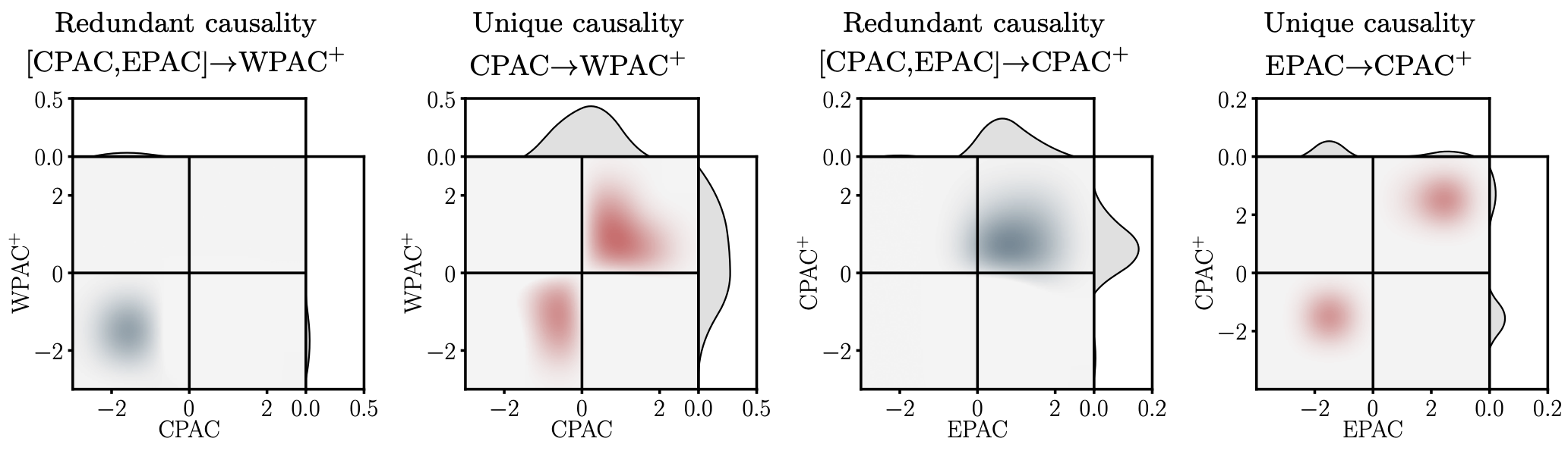
The main takeaway is that the causal signal is not uniform. It is strongest in specific regimes, concentrating when Pacific anomalies are coherent (variables moving above or below their means together), while becoming weak or absent in “mixed-sign” situations where the basin is not aligned.

A new lens for understanding complex systems

More broadly, our framework provides a new lens for understanding complex systems from observational data: it does not just tell us whether variables are linked, but when that link is active and how different sources combine to drive an outcome. We hope this state- and interaction-resolved view of causality will help turn large datasets into clearer scientific explanations across disciplines.

Revealing how system states shape causal interactions